Methods

For a more thorough description of the methods, see the full paper at https://doi.org/10.1038/s41597-023-02485-5 .

Model Selection

We selected the CMIP6 GCMs based on three criteria-

1. Overall skill: We selected the models that ranked higher based on a comprehensive skill assessment over the conterminous United States [ Ashfaq et al., 2022 ].
2. Data availability: We calculated deltas based on air temperature, near-surface air temperature, skin temperature, relative humidity, sea-surface temperature. The models that have these variables available at monthly scale for both ssp245 and ssp585 scenarios were selected. We use 1-5 ensemble members per model based on the availability.
3. Independent models (one model/institute): Models from same institute tend to perform similarly. Therefore, we selected one model/institute even if multiple models have high ranking.

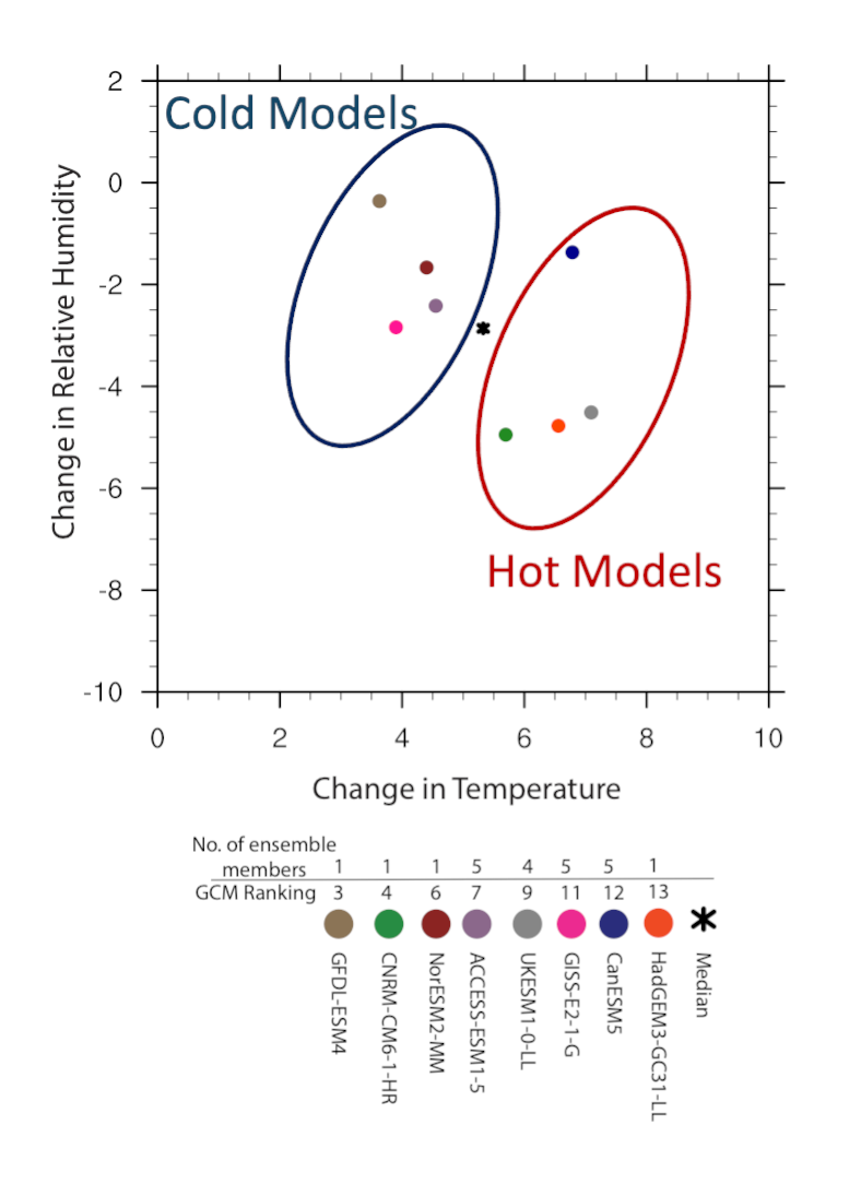
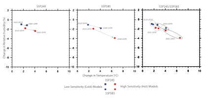
The selected models and ensembles used are summarized in Table 1. The selected models were further grouped into high and low sensitivity models based on the changes projected in temperature by the ensemble mean in SSP245 and SSP585 scenarios (e.g., Figure 1). The changes projected by the mean of two sets (high and low sensitivity) of models for two future time periods are shown in Figure 2.

Data Processing and Delta Calculation

All the data processing was done for monthly data for air temperature, near-surface air temperature, skin temperature, relative humidity, sea-surface temperature for SSP245 and SSP585 scenario, the data from 1979-2014 was obtained from the historical experiments.

1. Each ensemble member was remapped to a common 1-degree latitude-longitude grid. Additionally, the atmospheric variables (air temperature and relative humidity) were interpolated to ERA-5 atmospheric levels.
2. Ensemble mean for each of CMIP6 models was created using the ensembles listed in Table 1. The model mean for low and high sensitivity models was then calculated based on their ensemble means.
3. Moving average was calculated for each year from 1979 to 2099. 11 years centered on a given year were used to calculate moving average (e.g., the average for January of 1980 will be moving average of January from 1975-1985). Since the data is available until 2100, the window was reduced to 9,7,5,3 years as we approached 2099.
4. Monthly deltas were calculated for each year in 2019-2059 and 2059-2099 period with respect to the corresponding year in 1979-2019. The first year was used as spin up in each experiment.
5. Monthly deltas were interpolated to 3-hourly levels using linear interpolation between two months. The 3-hourly deltas were then added to the ERA-5 reanalysis to perform the future simulations.

Figure 1: Scatter plot showing the change in temperature versus change in relative humidity for late 21st century under SSP585 scenario with respect to historical period. The change is calculated as the difference between 2060 to 2099 and 1980 to 2019 in the ensemble mean of each of the eight CMIP6 models. Models with high/low temperature sensitivity are show in red /blue oval

Figure 2: Scatter plots showing the change in temperature versus change in relative humidity for near term (2020-2059) and late (2060-2099) 21st century in low and high sensitivity model mean under a) SSP245 and b) SSP585 scenario with respect to the historical period (1980-2019). The change in both SSP245 and SSP585 is shown together in panel c) for comparison. High/low sensitivity models are show in red and blue, changes during SSP585/SSP245 are shown circle/squares.

WRF Configuration and Testing

The Weather Research and Forecasting (WRF) model Version 4.2.1 [ Skamarock et al., 2019 ] was configured over a domain size of 425 × 300 grid points (Figure XX). WRF is a well-established, state-of-the-science, fully compressible, non-hydrostatic, mesoscale numerical weather prediction model. One reason for the robust use of WRF in the weather and climate modeling literature that it allows for multiple options for each physics parameterization, such as micro-physics, planetary boundary layer, radiation, and land surface processes. In the current section we describe our testing of multiple WRF parameterizations and options over one single year with the goal of finding a reliable model setup that produces acceptable biases across the CONUS. Following selection of the model configuration, we validate the model performance over the full 40-years historical period, in the next section. Here, we do not necessarily seek an optimal configuration as different configurations could produce the best performance for different regions or for different fields, such as water cycle components (e.g., precipitation and evapotranspiration), meteorological extremes, climatological means, etc. [ Ikeda et al. 2010 ; Rasmussen et al. 2011 , 2014a ; Liu et al. 2011 ; Liu paper; Stefan’s paper]. Neither are we seeking to quantify the value added by the increased resolution to the downscaled ERA5 reanalysis. Our goal is to find a reliable model configuration that reproduces historical climate with reasonable confidence, as a basis upon which the GCM-based ‘deltas’ can be implemented.

Our initial WRF parameterization setup follows recommendations by the National Center for Atmospheric Research (NCAR), which supports the WRF model and has run the model for real-time forecasting over the CONUS for years. These recommendations have been implemented in form of a combination of physics options (i.e., a physics suite) specific to the CONUS-scale application of WRF, starting in version 3.9. We further test two alternative parametrization combinations informed by literature precedents: Rahimi et al., 2022 and Liu et al., 2017 (Table 1). We note that for all the simulations, we used Noah LSM as the land surface model as it is the only land surface model in WRF compatible with the National Land Cover Data (NLCD) [40], the only available CONUS-scale land cover dataset with heterogeneous (with more than one urban land use/cover type) representation of urban areas. Representation of urban surfaces, with adequate fidelity, is important for two reasons: 1) urban areas are increasingly shown to have important implications for atmospheric moisture, wind, boundary layer structure, cloud formation, precipitation, and storms [Qian review paper]; 2) surface observations, especially over urban areas, are rarely assimilated in reanalysis datasets [ Kalnay and Cai, 2003 ; QIAN review paper], including ERA5. We further use the NLCD impervious surface data [41] and the single-layer urban canopy model (UCM) [43,44] for an accurate representation of urban cover (fraction of developed or built surfaces) and processes. UCM resolves urban canopy processes and the exchange of energy, moisture, and momentum between urban surfaces and the planetary boundary layer. The UCM parametrizes the three-dimensional nature of street canyon where it accounts for the shadowing, reflection, and trapping of the radiation and wind profiles [45].

Using the three parametrization combinations, we dynamically downscale ERA5 for 2009 to the 12 km CONUS domain. All the simulations use 39 vertical levels and daily sea-surface temperature (SST). Following reports of improved model performance and to prevent significant model drift over attempted long simulations [ Rahimi et al, 2022 ; Wang & Kotamarthi, 2013 ; Liu et al., 2017 ; Zobel et al., 2017 ], we apply spectral nudging to the temperature, geopotential height, and horizontal winds. To limit the exerted constraints, nudging starts from the PBL top, an approach well-established in the literature [ Spero et al., 2014 , 2018 ; Rahimi et al., 2022 ; Liu et al., 2017 ], up to the model top of 50 hPa. Spectral nudging parameters, the zonal and meridional grid-relative wavenumbers were set to 3 which constraints large scale phenomena (larger than ~1.5 km) while allowing for mesoscales and sub-synoptic scales such as convective systems to evolve freely.